Economic Affairs, Vol. 65, No. 1, pp. 23-30, March 2020
DOI: 10.30954/0424-2513.1.2020.4
©2020 EA. All rights reserved
A Comparative Analysis of Rural-Urban Migrants and NonMigrants in the Selected Region of Tamil Nadu, India
Revathy, N.*, Thilagavathi, M. and Surendran, A.
Department of Agricultural Economics, Centre for Agriculture and Rural development studies, Tamil Nadu Agricultural University, Coimbatore, Tamil Nadu, India
*Corresponding author: revathy.tnau14@gmail.com (ORCID ID: 0000-0002-6543-8957)
Received: 17-08-2019
Revised: 24-01-2020
Accepted: 29-02-2020
ABSTRACT
The study has assessed the impact of rural-urban migration by comparing migrant and non-migrant households in the Tiruppur district of Tamil Nadu. In this connection, a purposive sampling technique was used to select 80 migrant and 80 non-migrant respondents from the study region. Moreover, the study was employed decomposition analysis to understand the income difference between two groups with respect to migration. The estimated result shows that 65.35 percent of the income difference between migrant and non-migrant households due to migration. Also, noticed that comparatively migrants experience a better standard of living along with savings due to higher income and they did not have an idea of returning to agriculture. However, migration is an indication of unequal development of rural and urban which could be minimized by improvising rural living standards by creating employment opportunities, motivating entrepreneurship activities, supporting farming community with special reference to small and marginal farmers.
Highlights
 The study evaluated the impact of migration in terms of their economic condition. It stresses the need to develop the rural household standards to prevent the social rural-urban imbalance.
Keywords: Rural-urban migration, impact of migration, decomposition analysis, return migration
Migration is the movement by people from one place to another with the intentions of settling temporarily or permanently in the new location (Lee, 1966; Ekong, 2003). Migration occurs at a variety of scales: intercontinental (between continents), intracontinental (between countries on a given continent), and interregional (within countries). In larger countries like India and China, internal migration is more common than international migration (ILO, 2015). The increasing degree of industrialization, consequent increase in demand for labour, existence of informal sector activities, the scope for self-employment and above all the preparedness to accept any kind of job for an earning drive people towards urban areas (Hossain, 2001; Wheeler and Waite, 2003; Kees and Richard, 2004; Deshingkar, 2009; Sundaravaradarajan et al. 2011; Kishore, 2013). As the chances of crop failure e on these lands is very high due to prevalence of more than 50 percent of net cultivable area under rain-fed situation, where the rainfall pattern is also erratic in its nature, the farmers generally do not invest in external inputs like improved seeds, fertilizers and plant protection measures and end up with poor crop yields, even during normal years. This leads to low agricultural income, agricultural unemployment, and underemployment which are considered as basic factors pushing the migrants towards urban areas with greater job opportunities (Ranis, 2004; Farooq et al. 2005; Thorat et al. 2011; Vinayakam and Sekar 2013).
How to cite this article: Revathy, N., Thilagavathi, M. and Surendran, A. (2020). A comparative analysis of rural-urban migrants and non-migrants in the selected region of Tamil Nadu, India. Economic Affairs,65(1): 23-30.
In India, migration is mostly influenced by social structures and patterns of development. The development policies of the state governments have not been able to check the process of migration. Uneven development is the main cause behind migration (Skeldon, 2000; Dev, 2014; Nair, 2014). In India, nearly 29 percent of the persons were migrants and the migration rate (proportion of migrants in the population) in the urban areas (35 percent) was far higher than the migration rate in the rural areas (26 percent). Among the migrants in the urban areas, nearly 59 percent migrated from the rural areas and 40 percent from urban areas. The reason for migration for male migrants was dominated by employment-related reasons, in both rural and urban areas. Nearly 29 percent of rural male migrants and 56 percent of urban male migrants had migrated due to employment-related reasons. A higher percentage of the persons were found to be engaged in economic activities after migration, for males the percentage of workers increased from 51 percent before migration to 63 percent after migration in rural areas and from 46 percent to 70 percent in urban areas. Migration in India is predominantly to short distances, with around 60 percent of the migrants changing their residence within their district of birth and 20 percent within their state, while the rest move across the state boundaries (NSSO,2010).
Tamil Nadu is the second-largest economy in India and is one of the top industrialized and urbanized states of India with 48.45 percent of the population living in urban areas (Census of India, 2011). According to a census of India 2001, in Tamil Nadu, 94.30 percent of them have migrated within the state, of that 68.40 percent was intradistrict migration and 25.90 percent was inter-district migration. Coimbatore is one of the top 5 districts with higher in-migrants and Tiruppur is a part of Coimbatore in this period (Census of India, 2010). A higher percentage of the persons were found to be engaged in economic activities after migration (Anamica, 2010; Khatri 2007; Singh et al. 2011; Kaur, 2011; Basu and Faetanini, 2015), for males the percentage of workers increased from 51 percent before migration to 63 percent after migration in rural areas and from 46 percent to 70 percent in urban areas. (NSSO, 2010). With this background this paper analyses the impact of this rural-urban migration to reveal the benefits of migration on status of income, expenses, savings, debt, etc., and the impact on agriculture, by the direct investment made by migrants through their remittances and indirectly by overcoming debt position of the household which would support farming. Also, the intention of migrants on their interest in returning back to agriculture had been studied to ensure the farming community population.
Methodology
The influence of growing urban centers and industries on rural economies has been strongly felt most typically in Tiruppur which often called the "Banian city". Manufacturing of knitted products ranked 8th in terms of labour intensity (Das et al.2009) and this labor-intensive manufacturing sector attracted numerous labours, including migrants from nearby villages, different districts of Tamil Nadu and more recently from north Indian states as well. The textile industry provides employment to over six lakh people and a large portion of them i.e., about 75-80 percent of them are migrants (Trade Union, CITU). Thus Tiruppur district is selected purposively for the study. Migrants comprises of labours who work in textile industries of Tiruppur city and migrated from the agricultural sector and thus purposive sampling method was used in the selection of migrants.
There were 60 wards in Tiruppur city, from that two wards in each direction is chosen randomly and there come to a totally 8 wards. From each ward, 10 migrants who came from the agricultural sector have been chosen purposively. Thus there comes 80 migrants in total. Eighty Non-migrants were chosen purposively from respective villages of migrants and distribution of respondents were presented in Table 1 and 2. Therefore 160 is the total sample size. Primary data on the details required for the study were collected through personal and phone interview employing a pretested and well- structured questionnaire.
Decomposition analysis for income difference between Migrant and Non-migrant
The economic impact of migration is revealed through Blinder decomposition. The factors like age of the worker, education level, number of workers in the household, land size and marital status have been identified as important factors in determining the income level of migrant households. On the basis of these variables, wage equations were estimated and decomposed by using the technique of Blinder (1973) in the following manner:
Table 1: Distribution of migrant sample respondents in the Tiruppur District
Table 2: Distribution of non-migrant sample respondents from the migrant's native place
In Equations (1) and (2) above, the symbol' stands for migrants and 'n' for non-migrants. The symbol 'W' stands for household income measured in rupees. The estimated coefficients from such a model approximately measure the proportionate effect on incomes by the change in the right side variable 'X', which is a vector of the measured characteristics of the households such as age, education level, number of workers in the household, landholdings size and marital status of the respondents. The vector of regression coefficient 'α' (alpha) reflects the return that the market yields to a unit change in endowments and the error term 'ε' reflects the measurement error as well as the effect of the unmeasured or unobserved factors.
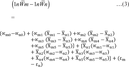
The Blinder Decomposition simply shows that equation 1 & 2 can be expanded as,
Where,
h Wm =log of migrant's annual income (₹/year)
h Wn = log of non-migrant's annual income (₹/ year)
𝛼m0 = Intercept of migrant equation
𝛼n0 = Intercept of the non-migrants equation Xm1 = Age of migrant (years)
Xm2 = Educational level of migrants (years)
Xm3 = Number of workers in migrant households (numbers)
Xm4 = Size of land holdings of migrant (ha)
Xm5 = Marital status of migrant (dummy variable = 1: married, 0: unmarried)
Xn1 = Age of non-migrant (years)
Xn2 = Educational level of non-migrants (years)
Xn3 =Number of workers in non-migrant households (numbers)
Xn4 = Size of land holdings of non-migrant (ha)
Xn5 = Marital status of migrant (dummy variable=1: married, 0: unmarried)
εm = Error term of migrant equation
εn = Error term of non-migrant equation
This is the overall income gap in the group of migrants (m) and non-migrants (n). The income gap is divided into two components: one is the portion attributable to differences in the endowments of income-generating characteristics (Xm- Xn ) )evaluating at the group 'M' returns (𝛼m). The second portion is attributable to the difference in the returns (𝛼m- 𝛼n) that groups 'm' and 'n' get for the same endowment of income-generating characteristics (Xn). This component is often taken as a reflection of discrimination or income differentials.
RESULTS AND DISCUSSION
Average monthly income of sample respondents: Income was the prime factor seeking for which migration takes place generally. The monthly household income of sample respondents is provided in Table 3. A higher on-farm and offfarm income of non-migrant households indicate the dependence of agriculture by non-migrants. The non-farm income of sample households was ₹ 16700 and ₹ 2350 for sample migrant and nonmigrant farm households, respectively. It implies the influence of migration on income of migrant among migrant households and lesser non-farm income among non-migrants indicates the poor employment opportunities in the rural areas. Average income between migrant and non-migrant households differs significantly and it concluded that the average income of migrant households (₹ 17868) was much higher than non-migrant households (₹ 7202).
Debt position: It is very much essential to assess the debt position of sample migrants before and after migration with regard to know about the influence of migration on changes in debt position. Hence it was estimated and presented in Table 3. It was noticed that there were increases in percent of sample migrant respondents free from debt position i.e. In the beginning, only 35 percent of the sample respondents did not have debt before migration and it was increased to 48.75 percent due to migration. This shows the power of migration in increasing the earning capacity of individuals and reducing the debt position of households.
Monthly Household Expenditure: Expenditure measures the economic standard of living and it was estimated from Table 3 that the monthly average expenditure of migrants was ₹ 11825.69 and non-migrants were ₹ 5661. Migrant expenditure was much higher than non-migrant, which implies that migrants had a better standard of living than non-migrants.
Savings Position: Savings amount can be used for the creation of assets and make use of money for better health, education and to meet out unforeseen circumstances, etc. The savings position of sample respondent households was estimated and presented in Table 3. The average monthly savings of migrants were higher than the non-migrants and this finding supports Lewis dual sector model according to which savings of workers moving to the industrial sector from agricultural would increase because of increased income level.
Return Migration: Return Migration is the voluntary movements of immigrants back to their place of origin. Even though migrants have moved to urban they are also having an idea to come back to villages after completing their commitments. Migrants' idea on return migration is provided in Table 4.
Table 3: Descriptive Statistics of the Sample Respondents
Figures in the parentheses indicate percentage to total.
Table 4: Return Migration According to Land Holding of Migrants
Figures in the parentheses indicate percentage to total.
The idea it was revealed from the table that, the agricultural labours do not want to return to agriculture and it is evident from the table that landholdings and return migration are directly related to each other. As the size of land holdings increases more there is an idea of returning to agriculture.
Income Determination between Migrants and Non-migrants: To delineate the impact of migrant's income on rural households income, the decomposition analysis was used by estimating the income equations for migrants and non-migrants separately and results are presented in Table 5. The regression coefficients have been used for calculating wage differentials due to personal endowments and structural differences. Both the equations show high values of R2 and variables in both the equation seems well specified. The high values of F indicate the overall significance of the model.
It could be seen from the table that in the case of non-migrant the coefficient of determinations (R2) was 0.68 which indicated that 68 percent of variation in the dependent variable was influenced by the explanatory variables which are included in the model. The significant F value of 34.97 indicates the goodness of fit. The dependent variable log of annual income is about 11.168. Explanatory variables like the educational level of the respondent, the number of workers in the household and the size of landholdings had a positive and significant influence at one percent level. One percent increase in the educational level of sample respondents, working population of household and land size would increase the income of non-migrants by 0.03, 0.55 and 0.10 percent, respectively.
In the case of migrant, the coefficient of determinations (R2) was 0.77 which indicated that 77 percent of variation in the dependent variable was influenced by the explanatory variables of the model. The significant F value of 54 indicates the goodness of fit. The dependent variable log of annual income is about 12.220. Explanatory variables like the educational level of the respondent and the number of workers in the household had a positive and significant influence at one percent level. One percent increase in the educational level of sample respondents and the working population of household would increase the income of migrants by 0.09 and 0.15 percent, respectively.
The absolute contribution of individual variables towards overall earnings differential between migrants and non-migrants is given in table 6. The endowment related factors of the workers like education, the number of workers in the household, size of land holdings contribute favourably in the case of migrants, whereas age and marital status favoured non-migrants.
Table 5: Decomposition Analysis Income determination model for Migrant and Nonmigrant Respondents
Note: *** indicates significant at 1 % level.
Further, the contribution of different factors towards the income difference between the two groups arises due to the differences in coefficients of the explanatory variables of the two-income equations. It is seen from the table that age, education and marital status contributed in favour of migrants.
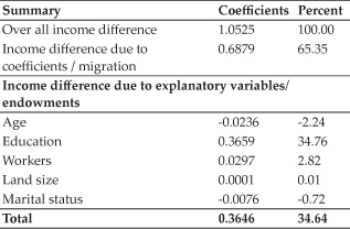
From table 7, the estimated result shows that 65.35 percent of the income difference between the migrant and non-migrant sample respondent households was due to the structural difference called migration. Whereas, the endowment differences contributed to 34.64 percent of income difference due to factors included in the model like age (-2.24 percent), education (34.76 percent), workers population (2.82 percent), land size (0.01 percent) and marital status (-0.72 percent). The average annual income of migrant was ₹ 214419.3 and non-migrant were ₹86424.3. Out of the total difference of ₹ 127995, the difference due to superior endowment of migrants about ₹ 44337.46 and difference due to migration was ₹ 83644.73 per annum.
Table 6: Decomposition of Income Differentials between Migrant and Non-migrants
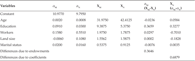
Table 7: Decomposition of Total Differences in Income of Migrant and Non-migrant respondents
CONCLUSION
The study analysed the impact of rural-urban migration by comparing income, expenditure and savings position of migrants and non-migrants and it was found that migrants had higher income, higher expenses and better savings implicating the betterment of life of migrants because of migration. The debt position of migrants had drastically reduced (to 51.18 percent) after migration because of higher income. As migrants started earning higher wages from migration, it helps them in savings and creation of assets. Migrant households made an investment in jewels, purchasing of vehicles, and housing and to a lesser extent in agriculture. It was also noted that almost three fourth of the migrants did not want to return to the agriculture sector which has to considered alarming. The study stresses the need for the creation of employment opportunities in rural areas that will decrease the rate of migration and also will increase the economic standard of non-migrant households.
REFERENCES
Anamica, M. 2010. Migration behaviour of dryland farmers - an expost facto study. Thesis M.Sc.(Ag.). Tamil Nadu Agricultural University, Coimbatore.
Basu, M. and Faetanini, M. 2015. Domestic Remittances in India: Estimates and Uses. Report for Gender youth migration, sub community of gender community, UN solution exchange, UNESCO.
Blinder, A.S. 1973. Wage discrimination: reduced form and structural estimates. Journal of Human Resources, pp. 436455.
Census of India. 2011. Migration tables in 2011 census, Government of India
Das, et al. 2009. The Employment Potential of Labourintensive Industries: An Appraisal of India's Organised Manufacturing. Working Paper 236, ICRIER, New Delhi.
Deshingkar, P. 2009. Circular Migration in India. Policy Brief No 4. World Development Report.
Dev, M. 2014. Small farmers, challenges and opportunities. Working paper no.14, Indira Gandhi Institute of Development Research, Mumbai, India.
Ekong, E.E. 2003. Rural sociology: An introduction and analysis of rural Nigeria. 2nd edition, Uyo, Nigeria, Dove educational publishers.
Farooq, M. et al. 2005. Determinants of Migration in Punjab, Pakistan: A Case Study of Faisalabad Metropolitan. Journal of Agriculture & Social Sciences, 1 (3): 280-282.
Hossain, M.Z. 2001. Rural-urban migration in Bangladesh, a micro-level study. 24th IUSSP General Conference, Salvador, Brazil.
ILO Global estimates on migrant workers 2015. Report of International labour Organisation.
Kaur, B. et al. 2011. Causes and Impact of Labour Migration: A Case Study of Punjab Agriculture. Agricultural Economics Research Review, 24 : 459-466.
Kees and Richard. 2004. Climate Change and Displacement in northwest Ghana, submitted for EACH-FOR Project.
Khatri, S.K. 2007. Labour migration, employment and poverty alleviation in South Asia. World bank report.
Kishore, Krishna. 2013. Labor Migration - A Journey from Rural To Urban. Journal of Business Management & Social Sciences Research, 2 (5): 61-66.
Lee, Everett. 1966. A Theory of Migration. Demography, 3 (1): 47-57.
Nair, Indira.. 2014. Challenges of Rural development and Opportunities for providing sustainable livelihood. International Journal of Research in Applied, Natural and Social Sciences, 2 (5): 111-118.
National sample survey organization, 64th round. 2010. Migration in India. National sample survey organization. Report No. 533. Ministry of Statistics and Programme Implementation, Government of India, New Delhi.
Ranis, G. 2004. Arthur Lewis's contribution to development thinking and policy. Manchester School, 72 (6): 712-723.
Singh N.P et al. 2011. Labour Migration in Indo-Gangetic Plains: Determinants and Impacts on Socio-economic Welfare. Agricultural Economics Research Review, 24 : 449458.
Skeldon, Ronald. 2000. Population mobility and HIV vulnerability in South East Asia: An assessment and analysis. UNDP South East Asia HIV and Development Project.
Sundaravaradarajan, K.R. et al. 2011. Determination of Key Correlates of Agricultural Labour Migration in Less Resources Endowed Areas of Tamil Nadu. Agricultural Economics Research Review, 24 : 467-472.
Thorat, V.A. et al. 2011. Impact of migration on rural economy of Konkan region. Agricultural Economics Research Review,24.
Vinayakam, K. and Sekar, S.P. 2013. Rural To Urban Migration in an Indian Metropolis: Case Study Chennai City. IOSR Journal of Humanities and Social Science, 6 (3): 32-35.
Wheeler, R. and Waite, M. 2003. Migration and Social Protection: A Concept Paper. Working Paper T2. Institute of Development Studies, Sussex.